I picked up the MAKE Rovera 2WD Arduino Robot Kit the other week and have been putting it together and checking it out. The kit comes with the book Make an Arduino-Controlled Robot that has the directions for construction and multiple projects (e.g., line following, edge detection, obstacle avoidance, etc.). There’s also a very similar 4 wheel drive kit that uses the same book, Arduino, motor controller, etc.

There’s code you can download from the net for each project, and the author walks through and explains the code in the included book. I like that the author talks about good practices like modular development in the book, and explains some of the nuances of using global variables with tabs when using the arduino IDE.
The kit’s primary components are the robot chassis, motors, and wheels from DF Robot, the Adafruit Motor Control Shield kit, a servo and Ping ultrasonic sensor, some IR sensors, and an Arduino Leonardo.
The kit assembles easily (but see “issues” below). Certainly it takes less than a day, and most of that is soldering the components and connectors on the motor shield. As someone who hasn’t done extensive soldering, I can say that soldering the parts on the motor shield kit was not difficult.

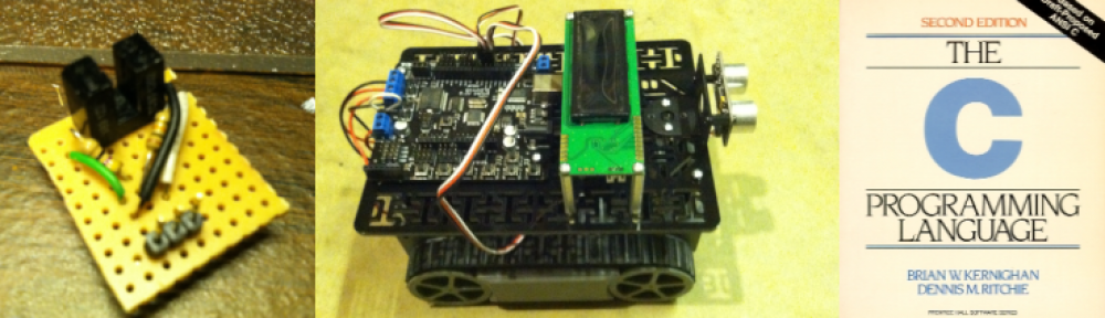
The physical assembly was even easier. I wasn’t sure of the best way to connect the sensors to the motor shield. The kit provides ribbon cable and some connectors (and the wrong type of prototype board that doesn’t match the strip board in the instructions). I decided the best way was to put together some 3 wire connectors using pre-crimped wires and 3×1 connector housings, as shown below:

Cables I substituted to connect the IR sensors.
At first I thought I’d just use some PWM cables I had lying around, but the positive and negative terminals are flipped between the IR sensors and the slots on the motor control shield, so you need to make sure to wire the connectors correctly, however you do it.
The Leonardo arduino board can be a bit ornery when first loading drivers. I had no trouble on one of my PCs, but I had to manually load the drivers on an old laptop (even though it’s running Windows 7. That’s not any fault of the kit, there’s a lot of discussion on line about this issue with the Leonardo board.
Once you have the robot assembled for the first time, you can run a simple test program that spins the robot. That verifies the basic functions. The next program in the book, the HelloRobot program, fully tests out the motor controller,

The assembled robot. Just need to connect the IR sensors and it’s ready to test.
IR sensors, etc., so it’s a good test that you put everything together correctly. I’m happy to report that once I fixed plugging the IR sensors into the wrong port (my bad), everything worked great.
That’s it for the initial build. Part 2 later, when I start checking out the functionality.
Initial Bottom Line: I recommend this kit, provided you have at least a little hobby experience with electronics and arduinos — a “practiced novice.” The troubles some have with a reliable Leonardo connection to a PC, the slight discrepancies between the kit as provided and the book, and the minor other inconsistencies in the book may, when combined, make this a frustrating experience if it’s a very first introduction to this world.
Issues:
- Be sure to check the on-line errata. It’s hard, just from the description in the book, to see how to wire up the trickle charge capability for rechargeable batteries. You can figure it out, but it’s not clear.
- The strip board described in the book to mount the IR sensors for line following wasn’t provided. Instead, another style of PC board was provided that doesn’t really work as intended.
- Read the book before building. In some sections, it begins to describe what seems like the next step, then after that step, points out it’s actually easier to do things in a different order! That’s annoying.
- Not the kit maker’s fault, but it would have been great if the +, -, and signal pins on the IR sensor were in the same order as the female headers used on the Adafruit motor shield, since then you could just use a standard PWM cable to connect them. Instead, the + and – are switched. Instead, the kit provides ribbon cable, which, with some soldering, can be used. I’m going to use some pre-crimped wires and crimp housings.
- It’s clear that the code, kit, and book went through some revisions during development, and not everything lines up. For example, one part of the HelloRobot section in the book says the robot will spin counter-clockwise when you trigger either IR sensor, while a page or two later, it says it will turn away from the triggered sensor (clockwise for left sensor, counterclockwise for right). The latter is correct. For software issues, when in doubt, read the actual code.
- If you’re looking to do navigation other than line following, you’ll need to be adding more to the robot. There are no wheel encoders even for basic dead reckoning, so the robot has no idea where it is. I’ve already played around with a home built robot that used a compass and wheel encoders, but no infrared sensors for edge detection or line following, so this was fine with me, but it’s something to be aware of.